Statistics

A Math? A Science? An Art? Or Something Else?

Isaac Quintanilla Salinas

Statistical Warning

Statistics

menti.com 2449 3348

Statistics

• With an increasing use of data to make decisions, Statistics has been essential for processing large amounts of data to byte-size information

• Statistics is also known as

  • Data Science

  • Machine Learning

  • Artificial Intelligence

• So for today, we’re asking: what is Statistics?

What does Google say?

UC Irvine

Statistics is the science concerned with developing and studying methods for collecting, analyzing, interpreting and presenting empirical data.

Wikipedia

Statistics is a mathematical body of science that pertains to the collection, analysis, interpretation or explanation, and presentation of data, or as a branch of mathematics.

What does AI say?

ChatGPT

Statistics is a branch of mathematics and a field of study that deals with the collection, analysis, interpretation, presentation, and organization of data.

Google Bard

Statistics is the science of collecting, analyzing, interpreting, and presenting data.

What do researchers say?

• Anthropologist
• Microbiologist
• Sociologist
• Political Scientist
• Ecologist
• Mathematician

Objectively interpreting data to make meaningful inferences about our predictions.

Whatever the statistician says.

Gathering the narratives of individuals, groups, or society and telling a story about their past, present, or future. The numbers paint a picture worth many words.

Using numbers to try to explain behaviors and/or patterns in our world.

Statistics is the way to make sense of the natural world by taking data we collect to identify patterns between variables, and applying statistical theory to make sure we are taking the right approach to data collection and analysis. Also, assess patterns to see if they are reproducible and provide a logical explanation that makes biological sense.

Statistics is the study of data, patterns, and trends.

What is it?

Math

Science

What does a Statistician say?

It is the study of variation and randomness!

Using mathematics, we model randomness to characterizes commonality and variation!

Using science, we systematically refine models to better fit randomness in data!

Using art, when it all eventually fails!

When it fails?!?!

Statistics Mantra - George Box

All models are wrong,

some are useful!

What is the formal definition of Statistics?

Statistics is both the development of mathematical models to be used in real-world data and the analysis of data using existing models.

Probability Models

• Model observations that follow a new data generating process

• Understand its properties

• Develop new probability distributions

• Known as Probability Theory

• Researcher is a Probabilist or Mathematical Statistician

Data Analysis

• Model data with a known probability model

• Account for sources of variation and bias

• Account for violations of independence and randomness

• Known as Statistician or Data Scientist

What’s the goal of a Statistician?

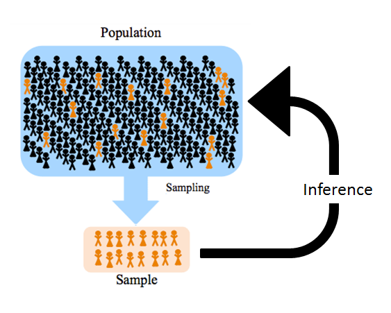
INFERENCE

Use our sample data to understand the larger population.

The data will tell us how the population generally behaves.

The data will guide us in the differences in units.

Data will tell us if there is a signal or just noise.

menti.com 2449 3348

Was the word cloud a scientific study?

YES!

We sampled a population!

Data was collected!

Data was summarized!

Another Word Cloud

Conducting Inference

Are we seeing something or is it just noise???

Are we seeing something different from what was expected? Or is it due to random chance?

Hypothesis Testing

1. Set up the Null and Alternative Hypothesis
2. Construct a test statistic based on the null hypothesis
3. Construct a distribution of the test statistic based on probability theory
4. Compute the probability of observing the test statistic
5. Make a decision based on the probability

What if we cannot construct the distribution?!?!

We bring out the Monte Carlo methods!

Monte Carlo Methods

• Monte Carlo Methods are used to construct a distribution function of an obscure test statistic
• We simulate a large number of data sets based on the null hypothesis
• We construct a test statistic for each fake data set and the real one
• We count how many data sets produce a test statistic that is more extreme than the real test statistic
• \(p=\#\ of\ extreme\ data\ sets\ /\ all\ data\ sets\)

Overview of Research

1. Ask a question about a population
2. Collect data from a sample
3. Construct and test a hypothesis
4. Draw conclusion about the population
5. Refine your question and methodology

So, what is Statistics?

For you baby, I’ll be anything

My Research

My Research

Generalized

Time-Varying

Joint Longitudinal-Survival Models

menti.com 2449 3348

menti.com 2449 3348

Joint Models

Longitudinal

• The analysis of repeated measurements

• Adjusting for extra correlation

• ie: Following a patient and collecting data at different time points

Survival

• The analysis of time-to-event data

  • Event can be anything

• Accounting for censoring

  • When information is not complete

  • Don’t know the whole time

• ie: Following a newly diagnosed cancer patient to death

Modelling them Jointly

• We can follow a newly-diagnosed patient longitudinally until the time-to-event occurs

• We can use the longitudinal outcome to explain the survival rate of diseases

• We can use the survival model to account for missing not at random in patients

Case Study

A patient is diagnosed with cancer, we want to know if any biomarkers can explain the survival rate of the disease.

Are there biomarker levels, that can increase the probability of not surviving the next month or year?

If so, can we do something about it to increase their chances of survival.

Data

With \(n\) participants, each \(i^{th}\) participant has:

Longitudinal Data

• \(n_i\) repeated measurements

• \(t_{i}=(t_{i1}, t_{i2}, \cdots, t_{in_i})^\mathrm T\)

• \(Y_i=(Y_{i1}, Y_{i2}, \cdots, Y_{in_i})^\mathrm T\)

• \(X_{ij}=(X_{ij1}, X_{ij2}, \cdots, X_{ijk})^\mathrm T\)

Survival Data

• \(T_i\): Observed time

• \(\delta_i\): Censoring status

Longitudinal Submodels

Our longitudinal outcome y can be represented in 2 components: a linear model and an error term. The linear \[\Large{Y_{ij} = m_i (t_{ij}) + \epsilon_i(t_{ij}),}\]

where

• \(m_i(t_{ij})=\boldsymbol{X}_{ij}^\mathrm T\boldsymbol \beta + \boldsymbol Z_{ij}^\mathrm Tb_i\)

• \(\boldsymbol X_{ij}\): design matrix

• \(\boldsymbol \beta=(\beta_1,\cdots,\beta_p)^\mathrm T\): regression coefficients

• \(b_i \sim N_q(\boldsymbol 0, \boldsymbol G)\)

• \(\epsilon_i(t_{ij})\): error term at time \(t_{ij}\)

• \(\boldsymbol Z_{ij}\): subset of \(\boldsymbol X_{ij}\)

• \(b_i=(b_{i1},\cdots,b_{iq})^\mathrm T\): random effects

• \(\epsilon_i(t_{ij}) \sim N(0, \sigma²)\)

Survival Submodels

\[\large{\lambda_i\{t|M_i(t),X_i\}=\lim_{\Delta\rightarrow 0}\frac{ P\{t\leq T_i <t+\Delta|T_i\geq t, M_i(t),\boldsymbol X_{i1}\}}{\Delta}}\] \[\large{\lambda_i\{t|M_i(t),\boldsymbol X_{i1}\}=\lambda_0(t)\exp\{\boldsymbol X_{i1}^\mathrm T\boldsymbol \gamma+\alpha m_i(t)\}}\]

where

• \(\lambda_0(t)\): baseline hazard function
• \(\boldsymbol X_{i1}\): design matrix at first time point
• \(\boldsymbol \gamma\): regression coefficients
• \(\alpha\): association coefficient
• \(M_i(t)\): history of the longitudinal outcome

Construction of the Joint Model

For an \(i^{th}\) individual:

\[P(T_i, \delta_i, \boldsymbol Y_i; \boldsymbol \theta)\]

\[ P(T_i, \delta_i, \boldsymbol Y_i; \boldsymbol \theta) \neq P(T_i, \delta_i; \boldsymbol \theta) P( \boldsymbol Y_i; \boldsymbol \theta) \]

What’s happening

Survival and Longitudinal

Random Effects

Construction of Joint Model

\[\begin{eqnarray} P(T_i, \delta_i, \boldsymbol Y_i; \boldsymbol \theta) &=& \int P(T_{i},\delta_{i}|b_{i};\boldsymbol \theta)P(\boldsymbol Y_{i}|b_{i};\boldsymbol \theta)P(b_{i};\boldsymbol \theta) db_i\\ & = & \int P(T_{i},\delta_{i}|b_{i};\boldsymbol \theta) \prod^{n_i}_j P(\boldsymbol Y_{ij}|b_{i};\boldsymbol \theta)P(b_{i};\boldsymbol \theta) db_i \end{eqnarray}\]

Estimation of parameters

In order to estimate the paramters (\(\theta\)), we must predict the random effects.

We must take care of the integral!

We either treat the random effects as parameters!

OR, we treat the random effects as missing!

Missing!?

Expectation-Maximization Algorithm

E-Step

Numerical techniques are used to target the random effects in the joint density function

• Gaussian Quadrature

• Laplace Approximation

• Monte Carlo Techniques

M-Step

A Newton-Raphson or other numerical techniques are used to maximize the expected likelihood function.

Estimation of Margin of Error

The standard errors of the parameters can be computed either as:

• Variance of the estimator, following probability model

• Using large sample theory of MLE, use the negative inverse Hessian matrix

Estimation of Margin of Error

The standard errors of the parameters can be computed either as:

• Variance of the estimator, following probability model

• Using large sample theory of MLE, use the negative inverse Hessian matrix

The Standard Errors are Biased due to misspecification of the random effects and baseline hazard function.

Bootstrapping

Bootstrapping can nonparametrically (or parameterically) compute the unbiased standard errors.

• Bootstrapping is conducted by sampling from the data set with replacement.

• Then a test statistic is constructed for each boot sample.

• The process is repeated many times until a distribution is constructed.

• Standard Errors (or Confidence Intervals) are obtained from the distribution.

• For joint models, the individual is sampled.

Questions

But Wait! There’s More!

What’s Statistics without a little …

Train of Thoughts

There are two train of thoughts on how to interpret estimates and probability.

One approach is the Frequentist approach.

The other approach is the Bayesian approach.

Both sides hate each other.

Frequentists

Frequentists

A frequentist, in the context of statistics, is an individual who adheres to the frequentist interpretation of probability and statistical inference.

Meaning probability is obtained by the repetition of multiple experiments.

Bayesians

Bayesians

A Bayesians, in the context of statistics, is an individual who adheres to the Bayesian interpretation of probability and statistical inference.

Probability is obtained by likelihood of an event to occur, given data and prior knowledge.

What am I (and people that have lives)?

Whatever gets the job done!

There is more, much more, but I will say this, in my statistical journey

www.inqs.info

isaac.qs@csuci.edu